Two Tools, Any Question: Building Axioma's MCP on a Semantic Layer

Axioma shows brands how AI engines like ChatGPT, Perplexity and Google’s AI see their sites: which pages AI agents visit, which brands the engines recommend, and how that lines up with Google Search Console demand. Its MCP (Model Context Protocol) server lets customers ask those questions in plain language from Claude or any other MCP client.

The tempting first design for an analytics assistant is text-to-SQL: give the model a tool that runs SQL over your warehouse and let it figure out the rest. It looks great in a demo and falls apart on real questions. It picks the wrong table out of three that look alike. It joins on a column that fans out and double-counts. It reinvents “AI visits” slightly differently every time, so its number never matches the dashboard. And you have to trust it to add the right WHERE clause so one customer never sees another customer’s rows. We never shipped that tool, and this post is about what we built instead.

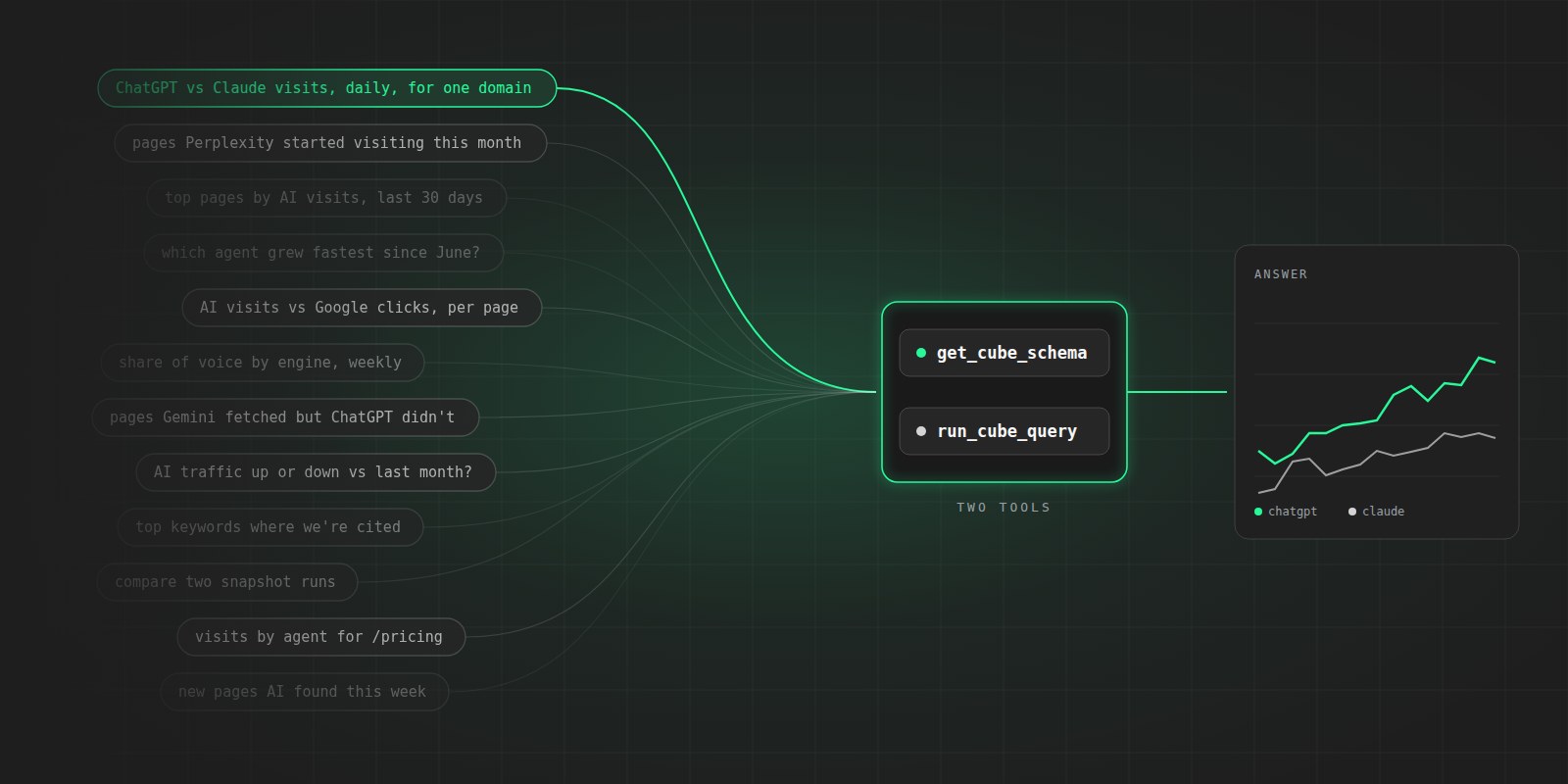
The usual fix is to take the query away from the model: one tool per chart. Traffic by engine. Top pages. Keyword breakdown. Share of voice over time. Safe, but every real customer question is slightly off from the menu. “ChatGPT vs Claude visits, daily, for one domain” is not “traffic by engine.” “Which pages did Perplexity start visiting this month that it didn’t visit last month” is not “top pages.” A one-tool-per-chart server either grows to hundreds of tools or keeps answering “I don’t have a tool for that.”

Before we wrote a line of the Axioma MCP, we wanted a third option: an assistant that is context-aware, that understands what data we have and figures out how to answer, without ever writing SQL. So the first two tools we built were not charts at all. One describes our data. The other queries it, through a semantic layer instead of raw tables. Instead of teaching the MCP hundreds of questions, we taught it how to ask questions safely.

The two tools that do the heavy lifting

Axioma’s analytics already run on Cube, a semantic layer that sits between our dashboards and BigQuery. Cube models data as cubes with named measures (things you count or sum), dimensions (things you group or filter by), and time dimensions. A dashboard chart is just a JSON query against that model.

That is the layer we exposed, through two tools:

• get_cube_schema returns the cubes the caller is allowed to see, with their descriptions. Ask for a specific cube and it returns that cube’s measures and dimensions, each with its own description.
• run_cube_query takes a Cube JSON query (measures, dimensions, filters, time range, order, limit) and runs it.

That’s the whole query surface. The model discovers what exists, decides what it needs, and composes the query itself. A question like “Compare ChatGPT vs Claude daily visits for example.com this month” becomes, with no dedicated tool:

We didn’t have to predict the question. We just had to make the data describe itself well enough that the model could find the answer.

This is also why most of the text-to-SQL problems go away. The model never touches a table or a join. Every join is defined once in the cube, so nothing fans out. Every measure is defined once, so “AI visits” means the same thing in the MCP as on the dashboard. And the model never writes the tenant filter, so there is no WHERE clause to get wrong. That filter is enforced in two layers: the MCP server adds a tenant_id filter to every query and forwards the caller’s JWT, then Cube’s checkAuth builds a security context from that token and queryRewrite enforces the tenant filter again.

What’s left is the model’s real decision: which cube, which members and which filter values. It can still get that wrong, picking the wrong cube or filtering on a value that doesn’t exist. It is the same kind of mistake as before, just in a much smaller space, and that is exactly the decision the descriptions are written to guide.

The schema is the prompt

The part that makes this work isn’t the tool. It’s the descriptions.

A schema that lists site_visits_daily, site_visits_with_gsc, and site_visits_with_trend with no explanation is useless to a model. It would guess, and it would guess wrong. So we treat every cube description and every field description as prompt engineering. They are written for the model, in the model’s terms: what the cube is, what a row means, which questions it answers, and, critically, when to pick a different cube instead.

In the cube definition, each of these is just a description field, written right next to the cube, measure or dimension it explains. Here is a simplified version of site_visits_daily:

# site_visits_daily.yml (illustrative example)
cubes:
  - name: site_visits_daily
    sql_table: analytics.site_visits_daily
    description: >
      Daily AI-agent visits: one row per day, domain, page and agent. The default cube for
      page-level traffic questions ("which pages did ChatGPT visit?"). Use site_visits_with_trend
      instead when the question asks for a change versus a previous period.
    measures:
      - name: ai_visits
        sql: visit_count
        description: >
          Times an AI agent fetched a page to answer a user's prompt (not training crawls).
          This is the headline number on the dashboard, so answers should use it by default.
    dimensions:
      - name: agent
        sql: agent_slug
        description: >
          The AI agent behind the visit. Values: chatgpt, claude, perplexity, gemini.
          Filter on these exact slugs.

Each description has a job. The cube’s description says what one row is and when to switch to site_visits_with_trend, so the model picks a cube by the shape of the user’s question. The ai_visits description marks it as the headline number on the dashboard, so the MCP’s answer matches what the customer already sees. And the agent description lists the exact values (chatgpt, claude, perplexity, gemini), so the model filters on slugs that exist instead of inventing ChatGPT-4.

It also keeps the MCP cheap to grow:

What we learned once real users arrived

The flexible primitive worked, but we also watched what people actually asked. A handful of questions dominated: per-engine traffic for a set of domains, top pages, top keywords, comparing snapshot runs. For those, composing a query from scratch every time was slower and occasionally inconsistent with the dashboard.

So we added named tools for the common questions. The important detail is how: each one is a thin recipe that builds a Cube query in code and runs it through the exact same run_cube_query path, with the same scoping, the same freshness window, and the same response trimming.

The freshness window exists because our data lands about four days late, so a plain “last 7 days” range would include days that aren’t fully loaded and would undercount. The shared path turns the default range into the seven most recent complete days, and the named tools build their ranges the same way. Response trimming happens on the way back: the server strips Cube’s extra metadata and shortens keys like site_visits_daily.ai_visits to ai_visits (unless two keys would collide), so the model gets smaller rows that are easier to read.

A query the model used to rebuild from the descriptions on every call is now code that can’t be miscopied.

The two layers complement each other. Named tools make the frequent questions fast and dashboard-exact. run_cube_query remains the escape hatch for everything else, and “everything else” is where an AI assistant earns its keep. When a customer asks the question nobody anticipated, the MCP doesn’t say “no tool for that.” It reads the schema, picks the cube the description points it to, and answers.

The takeaway

If you’re building an MCP server on top of an analytics stack, don’t start with text-to-SQL or with one tool per chart. Expose your semantic layer through a small number of general tools, then invest the saved effort in writing descriptions as if the model were a new analyst on their first day. Route between similar datasets explicitly. Name the dashboard-headline metric. List real enum values. Once real usage shows which questions dominate, add named tools for those, as recipes on the same query path rather than a replacement for it. Let the semantic layer own the joins, the metric definitions, and the access rules, so the model never has to.

The model turns out to be a very good analyst. It just needs a well-documented schema and a way to run a query.

Gal Ben Ami is a software engineer at Codo.